Tangent Lines

NOTE: This lesson is also available as executable worksheets on CoCalc. First, create an account and a project. Then you can copy these files to your project and start working right away. 07-tangent.ipynb (Jupyter Notebook) and 07-tangent.sagews (SageMath Worksheet).

In your experience with mathematics thus far, you have most likely come across the task of calculating the slope between two points. Whether you know it as "rise over run" or "change in y over change in x", the formula

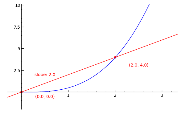
will give you the slope between points (x1, y1) and (x2, y2). So if, for instance, we were to calculate the slope between two points on f(x) = x³/2, say (0, 0) and (2, 4), we would find that by the formula, (4 - 0)/(2 - 0) gives us a slope of 2, as pictured on the following graph. For a purpose that will later be revealed, however, what if we were to find the slope of the function at a single point -- at (1, 1/2)? Such is the nature of the tangent line problem that we are about to explore, and is one of the basic questions of calculus.

Rather than simply generating a static graph this time, we'll be doing a bit of manipulation. In a new worksheet called 06-Tangent Lines, copy/paste the following code and evaluate it.

x1 = 0
x2 = 2

def f(x):
    return (x^3)/2

y1 = f(x1)
y2 = f(x2)

slope = (y2-y1)/(x2-x1)

p = plot(f(x), x, 0, 3)
pt1 = point((x1, y1), rgbcolor=(1,0,0), pointsize=30)
pt2 = point((x2, y2), rgbcolor=(1,0,0), pointsize=30)

d = 3
l = line([(x1-d, y1-d*slope), (x2+d, y2+d*slope)], rgbcolor=(1,0,0))

t1 = text("(%s, %s)" % (float(x1), float(y1)), (x1+0.5, y1-0.8), rgbcolor=(1,0,0))
t2 = text("(%s, %s)" % (float(x2), float(y2)), (x2+0.5, y2-0.8), rgbcolor=(1,0,0))
t3 = text("slope: %s" % float(slope), ((x1+x2)/2-0.5, (y1+y2)/2), rgbcolor=(1,0,0))

g = p+pt1+pt2+l+t1+t2+t3
g.show(xmin=0, xmax=3, ymin=-1, ymax=9)

1-2) Set the two x-coordinates
4-5) Create a function f(x) = x³/2
7-8) Calculate y1 and y2 based on the function f(x)
10) Calculate for slope
12) Plot f(x) on the interval [0, 3]
13-14) Draw (x1, y1) and (x2, y2) on the graph
16-17) Draw a secant line between the two points. 'd' affects the line's length
19-21) Display the location of the two points and the slope between them. (%s simply means, 'replace me with the value inside the following variable'.)
23-24) Combine the plot, points, line, and text and show them in a single graph.

In the graph, the straight line that passes through the two points is called a secant line -- we can say that it is an approximation of the function's slope at the point (1, 1/2), albeit not a very good one. What we want is a line tangent to the function at (1, 1/2) -- one that has a slope equal to that of the function at (1, 1/2).

To attain a better approximation of the slope at that point, let's try decreasing the distance between the two points at either side of it. In the first cell of your worksheet, change x1 to 0.5 and x2 to 1.5 and evaluate. Your graph should now look something like the following image:

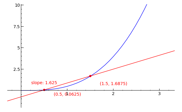
As you can see, the secant line in this graph still does not pass through the desired point of (1, 1/2), but at least we are getting closer. Now, try setting x1 as 0.999 and x2 as 1.001 and again evaluate the cell. Aside from looking cramped, what else can you observe about this graph? Ah ha! you surely say, it looks like the slope at (1, 1/2) is just about equal to 1.5000005. We could, of course, repeat this process in perpetuum, since when only a billionth of a unit separates the two points, there is little doubt that the calculated slope does, in fact, approximately equal the slope of f(x) = x³/2 at (1, 1/2).

Let us skip that theoretical headache, however, and consider a much faster (and even more accurate!) method. Look again at the formula for calculating slopes, this time in a slightly altered form:

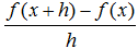
Rather than ignoring the relationship between the two points, as in the first form, this formula relies upon it. The symbol y2 is now f(x + h), and y1 is f(x). The major difference here, though, is that x2 has been replaced by the first x plus some change "h". The slope formula's premise still stands, however, as the new form does in fact calculate change in y over change in x.

So what can we do with this new formula, you ask? Well, what we would like to do is to make the change in x (designated by h) equal to zero in order to find the function's slope at a single point. Exchanging 0 for h does not work well, however, since that would make the formula simply (f(x + 0) - f(x))/0, which is not of much help (0/0 = ?). Let us consult SageMath, though, and see if there is a way to factor out h before setting it equal to zero. In a new cell, copy or type the following code.

def f(x):
    return (x^3)/2

var('x, h')
(f(x + h) - f(x))/h

1-2) Set f(x) as x³/2
4) Initialize variables x and h
5) Evaluate (f(x + h) - f(x))/h

The result should look like this: ((x + h)^3/2 - x^3/2)/h. With h still in the denominator, though, replacing it with zero would not be a good idea. Luckily, SageMath has a way for us to pull all variables from the denominator to the numerator, which is just what we need. In another cell, type and evaluate the following:

((f(x + h) - f(x))/h).rational_simplify()

The result should be (3*x^2 + 3*h*x + h^2)/2. Now that h is in the numerator, replacing it with zero will give us a formula for the function's slope at any value of x. To realize this result, add ".subs(h=0)" without the quotes to the end of rational_simplify() in the last entry and again evaluate the cell. And there you have it! By describing the change in x as a number 'h', we were able to simplify the formula for slope and replace h with zero in order to find that the slope of the function's tangent line at any x-coordinate is equal to 3*x²/2. This resulting expression is known as the derivative of f(x) = x³/2. You'll learn more about derivatives in the next section, but for now you should know that a function's derivative measures rate of change at a point.

To complete what we had originally set out to do, plug in a value of 1 for x, now, and you will see that the slope of the line tangent to the point (1, 1/2) on f(x) = x³/2 is 3/2. This confirms our earlier experimentation with numerical analysis in addition to being an exact solution. If we were to write an equation for this tangent line in slope-intercept form, it would be

.

It's very important to remember that the equation for a tangent line can always be written in slope-intercept or point-slope form; if you find that the equation for a tangent line is y = x^4*x²+e + sin(x) or some such extreme, something has gone (horribly) wrong. The slope of a tangent line will always be a constant.

You probably wouldn't be surprised to learn that this symbolic process involved a limit, specifically "the limit of (f(x + h) - f(x)))/h as h approaches zero." The slope that we found is also known as the derivative of f(x) at x=1. Look at how the tangent line lies against the graph of f(x) = x³/2:

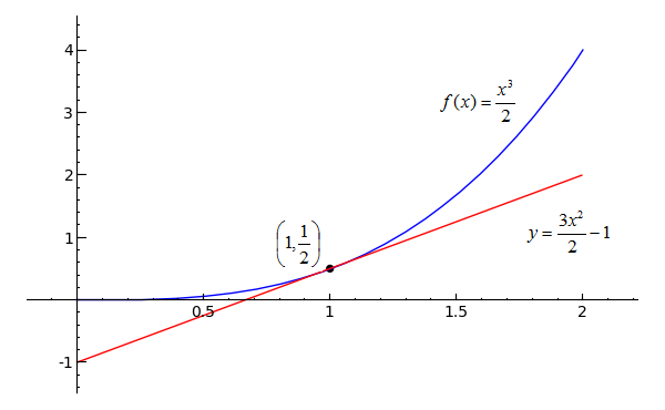
(plot(x^3/2, x, 0, 2)+plot(3*x/2-1, 0, 2, rgbcolor='red')+point((1, 1/2), \
	rgbcolor='black', pointsize=30)).show(xmin=0, xmax=2, ymin=-1, ymax=4)

1-2) Plot the original function with its tangent line and a point to show where they touch.

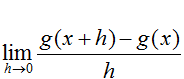
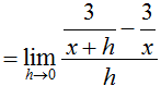
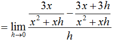
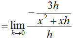
Now that we have an exact methodology for computing the slope of a tangent line, consider the function

What is the equation for the line tangent to (-2, g(-2))? The slope of the tangent line can be found using the function's derivative:

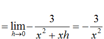
Plug in -2 for x, then write an equation for the tangent line:

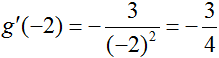, so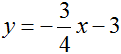

Here is another comparison:

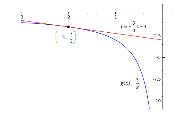
(plot(3/x, x, -3, 0)+plot(-3*x/4-3, -3, 0, rgbcolor='red')+point((-2, -3/2), \
    rgbcolor='black', pointsize=30)).show(xmin=-3, xmax=0, ymin=-10, ymax=0)

1-2) Plot the original function with its tangent line and a point to show where they touch.

Practice Problems

Use the limit process to find the equation of the line tangent to the indicated point.
1) at x=2.     Toggle answer
2) at x=-1.     Toggle answer
3) at t=5.     Toggle answer